RePsychLing Kliegl et al. (2010)

Author

Phillip Alday, Douglas Bates, and Reinhold Kliegl

Published

2022-09-27

Background

We take the kwdyz11.arrow dataset (Kliegl et al., 2010) from an experiment looking at three effects of visual cueing under four different cue-target relations (CTRs). Two horizontal rectangles are displayed above and below a central fixation point or they displayed in vertical orientation to the left and right of the fixation point. Subjects react to the onset of a small visual target occuring at one of the four ends of the two rectangles. The target is cued validly on 70% of trials by a brief flash of the corner of the rectangle at which it appears; it is cued invalidly at the three other locations 10% of the trials each.

We specify three contrasts for the four-level factor CTR that are derived from spatial, object-based, and attractor-like features of attention. They map onto sequential differences between appropriately ordered factor levels. At the level of fixed effects, there is the noteworthy result, that the attraction effect was estimated at 2 ms, that is clearly not significant. Nevertheless, there was a highly reliable variance component (VC) estimated for this effect. Moreover, the reliable individual differences in the attraction effect were negatively correlated with those in the spatial effect.

Unfortunately, a few years after the publication, we determined that the reported LMM is actually singular and that the singularity is linked to a theoretically critical correlation parameter (CP) between the spatial effect and the attraction effect. Fortunately, there is also a larger dataset kkl15.arrow from a replication and extension of this study (Kliegl et al., 2015), analyzed with kkl15.jl notebook. The critical CP (along with other fixed effects and CPs) was replicated in this study.

A more comprehensive analysis was reported in the parsimonious mixed-model paper (Bates et al., 2015). Data and R scripts are also available in R-package RePsychLing. In this and the complementary kkl15.jl scripts, we provide some corresponding analyses with MixedModels.jl.

Packages

Code

using Arrow
using AlgebraOfGraphics
using CairoMakie
using CategoricalArrays
using Chain
using DataFrames
using DataFrameMacros
using MixedModels
using MixedModelsMakie
using ProgressMeter
using Random
using StatsBase
using Statistics
using AlgebraOfGraphics: density
using AlgebraOfGraphics: boxplot

CairoMakie.activate!(; type="svg")
ProgressMeter.ijulia_behavior(:clear);

Read data, compute and plot densities and means

Code

dat = @chain "./data/kwdyz11.arrow" begin
  Arrow.Table
  DataFrame
  select(
    :subj =>
      (s -> categorical(string.('S', lpad.(s, 2, '0')))) => :Subj,
    :tar => categorical => :CTR,
    :rt,
    :rt => (x -> log.(x)) => :lrt,
  )
end
levels!(dat.CTR, ["val", "sod", "dos", "dod"])
describe(dat)

4 rows × 7 columns

	variable	mean	min	median	max	nmissing	eltype
	Symbol	Union…	Any	Union…	Any	Int64	DataType
1	Subj		S01		S61	0	CategoricalValue{String, UInt32}
2	CTR		val		dod	0	CategoricalValue{String, UInt32}
3	rt	370.426	150.1	358.6	705.7	0	Float64
4	lrt	5.886	5.0113	5.88221	6.55919	0	Float64

We recommend to code the levels/units of random factor / grouping variable not as a number, but as a string starting with a letter and of the same length for all levels/units.

We also recommend to sort levels of factors into a meaningful order, that is overwrite the default alphabetic ordering. This is also a good place to choose alternative names for variables in the context of the present analysis.

The LMM analysis is based on log-transformed reaction times lrt, indicated by a boxcox() check of model residuals. With the exception of diagnostic plots of model residuals, the analysis of untransformed reaction times did not lead to different results and exhibited the same problems of model identification (see Kliegl et al., 2010).

Comparative density plots of all response times by cue-target relation, Figure 1, show the times for valid cues to be faster than for the other conditions.

Code

draw(
  data(dat) *
  mapping(
    :lrt => "log(Reaction time [ms])";
    color=:CTR =>
      renamer("val" => "valid cue", "sod" => "some obj/diff pos", "dos" => "diff obj/same pos", "dod" => "diff obj/diff pos") => "Cue-target relation",
  ) *
  density(),
)

Figure 1: Comparative density plots of log reaction time for different cue-target relations.

An alternative visualization without overlap of the conditions can be accomplished with ridge plots.

To be done

For the next set of plots we average subjects’ data within the four experimental conditions. This table could be used as input for a repeated-measures ANOVA.

dat_subj = combine(
  groupby(dat, [:Subj, :CTR]),
  :rt => length => :n,
  :rt => mean => :rt_m,
  :lrt => mean => :lrt_m,
)

244 rows × 5 columns

	Subj	CTR	n	rt_m	lrt_m
	Cat…	Cat…	Int64	Float64	Float64
1	S01	val	330	413.332	6.01272
2	S01	sod	48	437.721	6.0682
3	S01	dos	47	443.366	6.08269
4	S01	dod	45	434.316	6.06079
5	S02	val	333	365.899	5.8751
6	S02	sod	47	396.149	5.95916
7	S02	dos	46	439.487	6.06949
8	S02	dod	48	441.042	6.06883
9	S03	val	336	371.446	5.90489
10	S03	sod	46	446.854	6.09464
11	S03	dos	48	471.302	6.14287
12	S03	dod	47	476.532	6.15706
13	S04	val	336	403.181	5.99124
14	S04	sod	48	446.075	6.09499
15	S04	dos	48	458.304	6.12005
16	S04	dod	48	441.054	6.08205
17	S05	val	310	358.714	5.84117
18	S05	sod	44	409.15	5.94934
19	S05	dos	45	457.493	6.10053
20	S05	dod	45	472.138	6.13361
21	S06	val	334	362.864	5.87953
22	S06	sod	48	368.123	5.89617
23	S06	dos	48	383.094	5.93601
24	S06	dod	48	367.973	5.88979
25	S07	val	326	407.497	5.98447
26	S07	sod	48	459.0	6.10927
27	S07	dos	42	486.502	6.17729
28	S07	dod	47	457.617	6.10471
29	S08	val	333	308.102	5.71815
30	S08	sod	48	323.875	5.76388
⋮	⋮	⋮	⋮	⋮	⋮

Code

boxplot(
  dat_subj.CTR.refs,
  dat_subj.lrt_m;
  orientation=:horizontal,
  show_notch=true,
  axis=(;
    yticks=(
      1:4,
      [
        "valid cue",
        "same obj/diff pos",
        "diff obj/same pos",
        "diff obj/diff pos",
      ],
    ),
  ),
  figure=(; resolution=(800, 300)),
)

Figure 2: Comparative boxplots of log response time by cue-target relation.

Mean of log reaction times for four cue-target relations. Targets appeared at (a) the cued position (valid) in a rectangle, (b) in the same rectangle cue, but at its other end, (c) on the second rectangle, but at a corresponding horizontal/vertical physical distance, or (d) at the other end of the second rectangle, that is \(\sqrt{2}\) of horizontal/vertical distance diagonally across from the cue, that is also at larger physical distance compared to (c).

A better alternative to the boxplot is a dotplot. It also displays subjects’ condition means.

To be done

Linear mixed model

contrasts = Dict(
  :CTR => SeqDiffCoding(; levels=["val", "sod", "dos", "dod"]),
  :Subj => Grouping(),
)
m1 = let
  form = @formula(lrt ~ 1 + CTR + (1 + CTR | Subj))
  fit(MixedModel, form, dat; contrasts)
end

Minimizing 254   Time: 0:00:00 ( 1.60 ms/it)
  objective:  -12782.373740584513

	Est.	SE	z	p	σ_Subj
(Intercept)	5.9358	0.0185	320.53	<1e-99	0.1441
CTR: sod	0.0878	0.0084	10.48	<1e-24	0.0582
CTR: dos	0.0366	0.0062	5.92	<1e-08	0.0274
CTR: dod	-0.0086	0.0060	-1.43	0.1515	0.0249
Residual	0.1920

VarCorr(m1)

	Column	Variance	Std.Dev	Corr.
Subj	(Intercept)	0.0207645	0.1440989
	CTR: sod	0.0033847	0.0581778	+0.48
	CTR: dos	0.0007531	0.0274423	-0.24	-0.15
	CTR: dod	0.0006221	0.0249410	+0.30	+0.93	-0.43
Residual		0.0368543	0.1919748

issingular(m1)

true

LMM m1 is not fully supported by the data; it is overparameterized. This is also visible in the PCA: only three, not four PCS are needed to account for all the variance and covariance in the random-effect structure. The problem is the +.93 CP for spatial sod and attraction dod effects.

first(MixedModels.PCA(m1))


Principal components based on correlation matrix
 (Intercept)   1.0     .      .      .
 CTR: sod      0.48   1.0     .      .
 CTR: dos     -0.24  -0.15   1.0     .
 CTR: dod      0.3    0.93  -0.43   1.0

Normalized cumulative variances:
[0.5886, 0.8095, 1.0, 1.0]

Component loadings
                PC1   PC2    PC3    PC4
 (Intercept)  -0.4   0.04   0.9    0.17
 CTR: sod     -0.6   0.4   -0.16  -0.68
 CTR: dos      0.33  0.91   0.06   0.23
 CTR: dod     -0.61  0.08  -0.41   0.68

Diagnostic plots of LMM residuals

Do model residuals meet LMM assumptions? Classic plots are

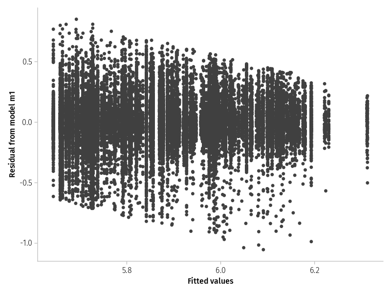
Residual over fitted
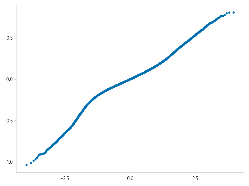
Quantiles of model residuals over theoretical quantiles of normal distribution

Residual-over-fitted plot

The slant in residuals show a lower and upper boundary of reaction times, that is we have have too few short and too few long residuals. Not ideal, but at least width of the residual band looks similar across the fitted values, that is there is no evidence for heteroskedasticity.

Code

CairoMakie.activate!(; type="png")
set_aog_theme!()
draw(
  data((; f=fitted(m1), r=residuals(m1))) *
  mapping(:f => "Fitted values", :r => "Residual from model m1") *
  visual(Scatter);
)

Figure 3: Residuals versus the fitted values for model m1 of the log response time.

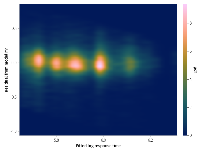
With many observations the scatterplot is not that informative. Contour plots or heatmaps may be an alternative.

Code

CairoMakie.activate!(; type="png")
draw(
  data((; f=fitted(m1), r=residuals(m1))) *
  mapping(
    :f => "Fitted log response time", :r => "Residual from model m1"
  ) *
  density();
)

Figure 4: Heatmap of residuals versus fitted values for model m1

Q-Q plot

The plot of quantiles of model residuals over corresponding quantiles of the normal distribution should yield a straight line along the main diagonal.

qqnorm(residuals(m1); qqline=:none)

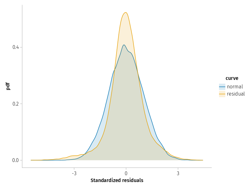
Observed and theoretical normal distribution

The violation of expectation is again due to the fact that the distribution of residuals is much narrower than expected from a normal distribution, as shown in Figure 5. Overall, it does not look too bad.

Code

let
  n = nrow(dat)
  dat_rz = DataFrame(;
    value=vcat(residuals(m1) ./ std(residuals(m1)), randn(n)),
    curve=vcat(fill.("residual", n), fill.("normal", n)),
  )
  draw(
    data(dat_rz) *
    mapping(:value => "Standardized residuals"; color=:curve) *
    density(; bandwidth=0.1);
  )
end

Figure 5: Kernel density plot of the standardized residuals from model m1 compared to a Gaussian

Conditional modes

Now we move on to visualizations that are based on model parameters and subjects’ data, that is “predictions” of the LMM for subject’s GM and experimental effects. Three important plots are

Overlay
Caterpillar
Shrinkage

Overlay

The first plot overlays shrinkage-corrected conditional modes of the random effects with within-subject-based and pooled GMs and experimental effects.

To be done

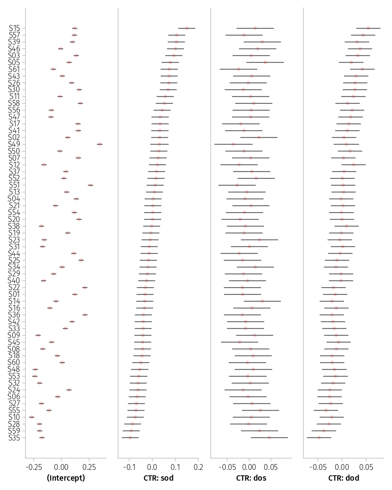
Caterpillar plot

The caterpillar plot, Figure 6, also reveals the high correlation between spatial sod and attraction dod effects.

Code

caterpillar!(
  Figure(; resolution=(800, 1000)), ranefinfo(m1, :Subj); orderby=2
)

Figure 6: Prediction intervals on the random effects for Subj in model m1

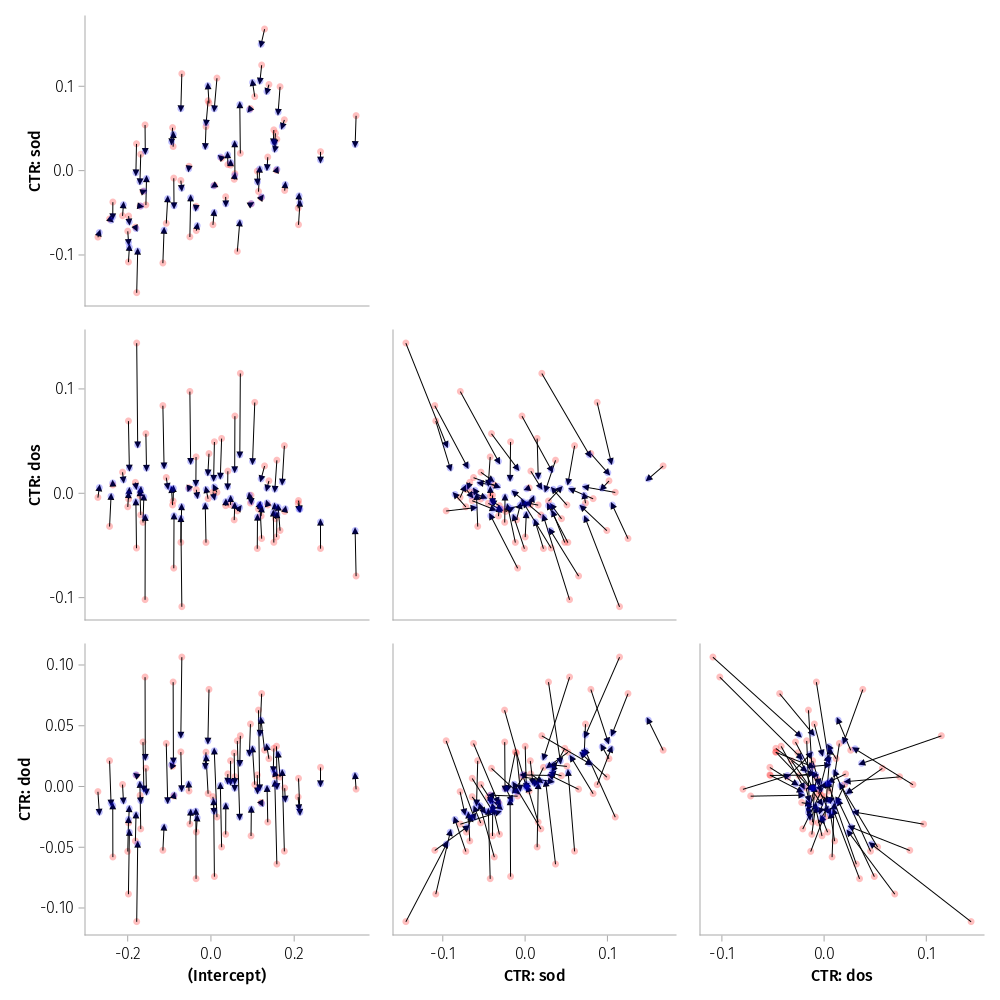
Shrinkage plot

Figure 7 provides more evidence for a problem with the visualization of the spatial sod and attraction dod CP. The corresponding panel illustrates an implosion of conditional modes.

Code

shrinkageplot!(Figure(; resolution=(1000, 1000)), m1)

Figure 7: Shrinkage plot of the conditional means of the random effects for model m1

Parametric bootstrap

Here we

generate a bootstrap sample
compute shortest covergage intervals for the LMM parameters
plot densities of bootstrapped parameter estimates for residual, fixed effects, variance components, and correlation parameters

Generate a bootstrap sample

We generate 2500 samples for the 15 model parameters (4 fixed effect, 4 VCs, 6 CPs, and 1 residual).

Code

Random.seed!(1234321)
samp = parametricbootstrap(2500, m1; hide_progress=true)
dat2 = DataFrame(samp.allpars)
first(dat2, 10)

10 rows × 5 columns

	iter	type	group	names	value
	Int64	String	String?	String?	Float64
1	1	β	missing	(Intercept)	5.93392
2	1	β	missing	CTR: sod	0.0864217
3	1	β	missing	CTR: dos	0.0488894
4	1	β	missing	CTR: dod	-0.0121838
5	1	σ	Subj	(Intercept)	0.13294
6	1	σ	Subj	CTR: sod	0.0497365
7	1	ρ	Subj	(Intercept), CTR: sod	0.604951
8	1	σ	Subj	CTR: dos	0.0278832
9	1	ρ	Subj	(Intercept), CTR: dos	-0.254321
10	1	ρ	Subj	CTR: sod, CTR: dos	0.0550145

nrow(dat2) # 2500 estimates for each of 15 model parameters

Shortest coverage interval

The upper limit of the interval for the critical CP CTR: sod, CTR: dod is hitting the upper wall of a perfect correlation. This is evidence of singularity. The other intervals do not exhibit such pathologies; they appear to be ok.

Code

DataFrame(shortestcovint(samp))

15 rows × 5 columns

	type	group	names	lower	upper
	String	String?	String?	Float64	Float64
1	β	missing	(Intercept)	5.89917	5.97256
2	β	missing	CTR: sod	0.0719311	0.104588
3	β	missing	CTR: dos	0.0251178	0.0491673
4	β	missing	CTR: dod	-0.0207176	0.0026829
5	σ	Subj	(Intercept)	0.116561	0.168571
6	σ	Subj	CTR: sod	0.0454958	0.0708402
7	ρ	Subj	(Intercept), CTR: sod	0.24378	0.712966
8	σ	Subj	CTR: dos	0.00921535	0.040977
9	ρ	Subj	(Intercept), CTR: dos	-0.870267	0.288412
10	ρ	Subj	CTR: sod, CTR: dos	-0.66917	0.562077
11	σ	Subj	CTR: dod	0.0144121	0.0386782
12	ρ	Subj	(Intercept), CTR: dod	-0.135087	0.740413
13	ρ	Subj	CTR: sod, CTR: dod	0.573681	0.999995
14	ρ	Subj	CTR: dos, CTR: dod	-0.896183	0.45778
15	σ	residual	missing	0.190558	0.193642

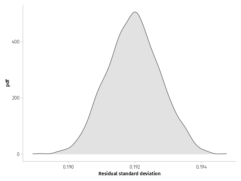
Comparative density plots of bootstrapped parameter estimates

Residual

Code

draw(
  data(@subset(dat2, :type == "σ", ismissing(:names))) *
  mapping(:value => "Residual standard deviation") *
  density();
)

Fixed effects (w/o GM)

The shortest coverage interval for the GM ranges from 376 to 404 ms. To keep the plot range small we do not inlcude its density here.

Code

labels = [
  "CTR: sod" => "spatial effect",
  "CTR: dos" => "object effect",
  "CTR: dod" => "attraction effect",
  "(Intercept)" => "grand mean",
]
draw(
  data(@subset(dat2, :type == "β" && :names ≠ "(Intercept)")) *
  mapping(
    :value => "Experimental effect size [ms]";
    color=:names => renamer(labels) => "Experimental effects",
  ) *
  density();
)

Figure 9: Comparative density plots of the fixed-effects parameters for model m1

The densitiies correspond nicely with the shortest coverage intervals.

Variance components (VCs)

Code

draw(
  data(@subset(dat2, :type == "σ" && :group == "Subj")) *
  mapping(
    :value => "Standard deviations [ms]";
    color=:names => renamer(labels) => "Variance components",
  ) *
  density();
)

Figure 10: Comparative density plots of the variance components for model m1

The VC are all very nicely defined.

Correlation parameters (CPs)

Code

let
  labels = [
    "(Intercept), CTR: sod" => "GM, spatial",
    "(Intercept), CTR: dos" => "GM, object",
    "CTR: sod, CTR: dos" => "spatial, object",
    "(Intercept), CTR: dod" => "GM, attraction",
    "CTR: sod, CTR: dod" => "spatial, attraction",
    "CTR: dos, CTR: dod" => "object, attraction",
  ]
  draw(
    data(@subset(dat2, :type == "ρ")) *
    mapping(
      :value => "Correlation";
      color=:names => renamer(labels) => "Correlation parameters",
    ) *
    density();
  )
end

Figure 11: Comparative density plots of the correlation parameters for model m1

Two of the CPs stand out positively. First, the correlation between GM and the spatial effect is well defined. Second, as discussed throughout this script, the CP between spatial and attraction effect is close to the 1.0 border and clearly not well defined. Therefore, this CP will be replicated with a larger sample in script kkl15.jl (Kliegl et al., 2015).

References

Bates, D., Kliegl, R., Vasishth, S., & Baayen, H. (2015). Parsimonious mixed models. arXiv. https://doi.org/10.48550/ARXIV.1506.04967

Kliegl, R., Kushela, J., & Laubrock, J. (2015). Object orientation and target size modulate the speed of visual attention. Department of Psychology, University of Potsdam.

Kliegl, R., Wei, P., Dambacher, M., Yan, M., & Zhou, X. (2010). Experimental effects and individual differences in linear mixed models: Estimating the relationship between spatial, object, and attraction effects in visual attention. Frontiers in Psychology. https://doi.org/10.3389/fpsyg.2010.00238