A large-scale designed experiment

Load the packages to be used.

Code

using AlgebraOfGraphics
using Arrow
using CairoMakie
using Chain
using DataFrameMacros
using DataFrames
using Effects
using MixedModels
using MixedModelsMakie
using ProgressMeter
using StandardizedPredictors
using StatsBase

datadir(paths::AbstractString...) = joinpath(@__DIR__, "data", paths...)
CairoMakie.activate!(; type="svg");
ProgressMeter.ijulia_behavior(:clear);

┌ Info: Precompiling Effects [8f03c58b-bd97-4933-a826-f71b64d2cca2]
└ @ Base loading.jl:1662

┌ Info: Precompiling StandardizedPredictors [5064a6a7-f8c2-40e2-8bdc-797ec6f1ae18]
└ @ Base loading.jl:1662

The English Lexicon Project (Balota et al., 2007) was a large-scale multicenter study to examine properties of English words. It incorporated both a lexical decision task and a word recognition task. Different groups of subjects participated in the different tasks.

Extracting data tables from the raw data

The raw data are available as an OSF project as Zip files for each of the tasks. These Zip files contain one data file for each participant, which has a mixture of demographic data, responses on some pre-tests, and the actual trial runs.

Parsing these data files is not fun – see this repository for some of the code used to untangle the data. (This respository is an unregistered Julia package.)

Some lessons from this:

• When an identifier is described as a “unique subject id”, it probably isn’t.
• In a multi-center trial, the coordinating center should assign the range of id’s for each satellite site. Failure of a satellite site to stay within its range should result in banishment to a Siberian work camp.
• As with all data cleaning, the prevailing attitude should be “trust, but verify”. Just because you are told that the file is in a certain format, doesn’t mean it is. Just because you are told that the identifiers are unique doesn’t mean they are, etc.
• It works best if each file has a well-defined, preferably simple, stucture. These data files had two different formats mushed together.
• This is the idea of “tidy data” - each file contains only one type of record along with well-defined rules of how you relate one file to another.
• If one of the fields is a date, declare the only acceptable form of writing a date, preferably yyyy-mm-dd. Anyone getting creative about the format of the dates will be required to write the software to parse that form (and that is usually not an easy task).
• As you make changes in a file, document them. If you look at the EnglishLexicon.jl repository you will see that it is in the form of scripts that take the original Zip files and produce the Arrow files. That way, if necessary, the changes can be undone or modified.
• Remember, the data are only as useful as their provenance. If you invested a lot of time and money in gathering the data you should treat it as a valued resource and exercise great care with it.
• The Arrow.jl package allows you to add metadata as key/value pairs, called a Dict (or dictionary). Use this capability. The name of the file is not a suitable location for metadata.

Trial-level data from the LDT

In the lexical decision task the study participant is shown a character string, under carefully controlled conditions, and responds according to whether they identify the string as a word or not. Two responses are recorded: whether the choice of word/non-word is correct and the time that elapsed between exposure to the string and registering a decision.

Several covariates, some relating to the subject and some relating to the target, were recorded. Initially we consider only the trial-level data.

ldttrial = Arrow.Table(datadir("ELP_ldt_trial.arrow"))

Arrow.Table with 2745952 rows, 5 columns, and schema:
 :subj  Int16
 :seq   Int16
 :acc   Union{Missing, Bool}
 :rt    Int16
 :item  String

with metadata given by a Base.ImmutableDict{String, String} with 3 entries:
  "title"     => "Trial-level data from Lexical Discrimination Task in the Engl…
  "reference" => "Balota et al. (2007), The English Lexicon Project, Behavior R…
  "source"    => "https://osf.io/n63s2"

The two response variables are acc - the accuracy of the response - and rt, the response time in milliseconds. There is one trial-level covariate, seq, the sequence number of the trial within subj. Each subject participated in two sessions on different days, with 2000 trials recorded on the first day.

Notice the metadata with a citation and a URL for the OSF project.

We convert to a DataFrame and add a Boolean column s2 which is true for trials in the second session.

ldttrial = @transform!(DataFrame(ldttrial), :s2 = :seq > 2000)
describe(ldttrial)

6 rows × 7 columns

	variable	mean	min	median	max	nmissing	eltype
	Symbol	Union…	Any	Union…	Any	Int64	Type
1	subj	409.31	1	409.0	816	0	Int16
2	seq	1687.21	1	1687.0	3374	0	Int16
3	acc	0.85604	0	1.0	1	1370	Union{Missing, Bool}
4	rt	846.325	-16160	732.0	32061	0	Int16
5	item		Aarod		zuss	0	String
6	s2	0.407128	0	0.0	1	0	Bool

Initial data exploration

From the basic summary of ldttrial we can see that there are some questionable response times — negative values and values over 32 seconds.

Because of obvious outliers we will use the median response time, which is not strongly influenced by outliers, rather than the mean response time when summarizing by item or by subject.

Also, there are missing values of the accuracy. We should check if these are associated with particular subjects or particular items.

Summaries by item

To summarize by item we group the trials by item and use combine to produce the various summary statistics. As we will create similar summaries by subject, we incorporate an ‘i’ in the names of these summaries (and an ‘s’ in the name of the summaries by subject) to be able to identify the grouping used.

byitem = @chain ldttrial begin
  groupby(:item)
  @combine(
    :ni = length(:acc),               # no. of obs
    :imiss = count(ismissing, :acc),  # no. of missing acc
    :iacc = count(skipmissing(:acc)), # no. of accurate
    :imedianrt = median(:rt),
  )
  @transform!(
    :wrdlen = Int8(length(:item)),
    :ipropacc = :iacc / :ni
  )
end

80,962 rows × 7 columns

	item	ni	imiss	iacc	imedianrt	wrdlen	ipropacc
	String	Int64	Int64	Int64	Float64	Int8	Float64
1	a	35	0	26	743.0	1	0.742857
2	e	35	0	19	824.0	1	0.542857
3	aah	34	0	21	770.5	3	0.617647
4	aal	34	0	32	702.5	3	0.941176
5	Aaron	33	0	31	625.0	5	0.939394
6	Aarod	33	0	23	810.0	5	0.69697
7	aback	34	0	15	710.0	5	0.441176
8	ahack	34	0	34	662.0	5	1.0
9	abacus	34	0	17	671.5	6	0.5
10	alacus	34	0	29	640.0	6	0.852941
11	abandon	34	0	32	641.0	7	0.941176
12	acandon	34	0	33	725.5	7	0.970588
13	abandoned	34	0	31	667.5	9	0.911765
14	adandoned	34	0	11	760.5	9	0.323529
15	abandoning	34	0	34	662.0	10	1.0
16	abantoning	34	0	30	848.5	10	0.882353
17	abandonment	35	0	35	734.0	11	1.0
18	apandonment	35	0	30	817.0	11	0.857143
19	abase	34	1	23	750.5	5	0.676471
20	abose	34	0	23	805.5	5	0.676471
21	abasement	33	0	17	850.0	9	0.515152
22	afasement	33	0	30	649.0	9	0.909091
23	abash	32	0	22	727.5	5	0.6875
24	adash	32	0	25	784.5	5	0.78125
25	abate	34	0	24	687.0	5	0.705882
26	abape	34	0	32	675.0	5	0.941176
27	abated	34	0	23	775.0	6	0.676471
28	agated	34	0	14	897.5	6	0.411765
29	abbess	34	0	7	837.5	6	0.205882
30	abbass	34	0	28	788.0	6	0.823529
⋮	⋮	⋮	⋮	⋮	⋮	⋮	⋮

It can be seen that the items occur in word/nonword pairs and the pairs are sorted alphabetically by the word in the pair (ignoring case). We can add the word/nonword status for the items as

byitem.isword = isodd.(eachindex(byitem.item))
describe(byitem)

8 rows × 7 columns

	variable	mean	min	median	max	nmissing	eltype
	Symbol	Union…	Any	Union…	Any	Int64	DataType
1	item		Aarod		zuss	0	String
2	ni	33.9166	30	34.0	37	0	Int64
3	imiss	0.0169215	0	0.0	2	0	Int64
4	iacc	29.0194	0	31.0	37	0	Int64
5	imedianrt	753.069	458.0	737.5	1691.0	0	Float64
6	wrdlen	7.9988	1	8.0	21	0	Int8
7	ipropacc	0.855616	0.0	0.911765	1.0	0	Float64
8	isword	0.5	0	0.5	1	0	Bool

This table shows that some of the items were never identified correctly. These are

filter(:iacc => iszero, byitem)

9 rows × 8 columns

	item	ni	imiss	iacc	imedianrt	wrdlen	ipropacc	isword
	String	Int64	Int64	Int64	Float64	Int8	Float64	Bool
1	baobab	34	0	0	616.5	6	0.0	1
2	haulage	34	0	0	708.5	7	0.0	1
3	leitmotif	35	0	0	688.0	9	0.0	1
4	miasmal	35	0	0	774.0	7	0.0	1
5	peahen	34	0	0	684.0	6	0.0	1
6	plosive	34	0	0	663.0	7	0.0	1
7	plugugly	33	0	0	709.0	8	0.0	1
8	poshest	34	0	0	740.0	7	0.0	1
9	servo	33	0	0	697.0	5	0.0	1

Notice that these are all words but somewhat obscure words such that none of the subjects exposed to the word identified it correctly.

We can incorporate characteristics like wrdlen and isword back into the original trial table with a “left join”. This operation joins two tables by values in a common column. It is called a left join because the left (or first) table takes precedence, in the sense that every row in the left table is present in the result. If there is no matching row in the second table then missing values are inserted for the columns from the right table in the result.

describe(
  leftjoin!(
    ldttrial,
    select(byitem, :item, :wrdlen, :isword);
    on=:item,
  ),
)

8 rows × 7 columns

	variable	mean	min	median	max	nmissing	eltype
	Symbol	Union…	Any	Union…	Any	Int64	Type
1	subj	409.31	1	409.0	816	0	Int16
2	seq	1687.21	1	1687.0	3374	0	Int16
3	acc	0.85604	0	1.0	1	1370	Union{Missing, Bool}
4	rt	846.325	-16160	732.0	32061	0	Int16
5	item		Aarod		zuss	0	String
6	s2	0.407128	0	0.0	1	0	Bool
7	wrdlen	7.99835	1	8.0	21	0	Union{Missing, Int8}
8	isword	0.499995	0	0.0	1	0	Union{Missing, Bool}

Notice that the wrdlen and isword variables in this table allow for missing values, because they are derived from the second argument, but there are no missing values for these variables. If there is no need to allow for missing values, there is a slight advantage in disallowing them in the element type, because the code to check for and handle missing values is not needed.

This could be done separately for each column or for the whole data frame, as in

describe(disallowmissing!(ldttrial; error=false))

8 rows × 7 columns

	variable	mean	min	median	max	nmissing	eltype
	Symbol	Union…	Any	Union…	Any	Int64	Type
1	subj	409.31	1	409.0	816	0	Int16
2	seq	1687.21	1	1687.0	3374	0	Int16
3	acc	0.85604	0	1.0	1	1370	Union{Missing, Bool}
4	rt	846.325	-16160	732.0	32061	0	Int16
5	item		Aarod		zuss	0	String
6	s2	0.407128	0	0.0	1	0	Bool
7	wrdlen	7.99835	1	8.0	21	0	Int8
8	isword	0.499995	0	0.0	1	0	Bool

Named argument “error”

The named argument error=false is required because there is one column, acc, that does incorporate missing values. If error=false were not given then the error thrown when trying to disallowmissing on the acc column would be propagated and the top-level call would fail.

A barchart of the word length counts, Figure 1, shows that the majority of the items are between 3 and 14 characters.

Code

let
  wlen = 1:21
  draw(
    data((; wrdlen=wlen, count=counts(byitem.wrdlen, wlen))) *
    mapping(:wrdlen => "Length of word", :count) *
    visual(BarPlot),
  )
end

Figure 1: Histogram of word lengths in the items used in the lexical decision task.

To examine trends in accuracy by word length we create a plot of the response versus word length using just a scatterplot smoother. It would not be meaningful to plot the raw data because that would just provide horizontal lines at \(\pm 1\). Instead we add the smoother to show the trend and omit the raw data points.

The resulting plot, Figure 2, shows the accuracy of identifying words is more-or-less constant at around 84%, but accuracy decreases with increasing word length for the nonwords.

Code

draw(
  data(@subset(ldttrial, !ismissing(:acc))) *
  mapping(
    :wrdlen => "Word length",
    :acc => "Accuracy";
    color=:isword,
  ) *
  smooth();
  figure=(; resolution=(800, 450)),
)

Figure 2: Smoothed curves of accuracy versus word length in the lexical decision task.

Figure 2 may be a bit misleading because the largest discrepancies in proportion of accurate identifications of words and nonwords occur for the longest words, of which there are few. Over 95% of the words are between 4 and 13 characters in length

count(x -> 4 ≤ x ≤ 13, byitem.wrdlen) / nrow(byitem)

0.9654899829549666

If we restrict the smoother curves to this range, as in Figure 3,

Code

draw(
  data(@subset(ldttrial, !ismissing(:acc), 4 ≤ :wrdlen ≤ 13)) *
  mapping(
    :wrdlen => "Word length",
    :acc => "Accuracy";
    color=:isword,
  ) *
  smooth();
  figure=(; resolution=(800, 450)),
)

Figure 3: Smoothed curves of accuracy versus word length in the range 4 to 13 characters in the lexical decision task.

the differences are less dramatic.

Another way to visualize these results is by plotting the proportion accurate versus word-length separately for words and non-words with the area of each marker proportional to the number of observations for that combinations (Figure 4).

Code

let
  itemsummry = combine(
    groupby(byitem, [:wrdlen, :isword]),
    :ni => sum,
    :imiss => sum,
    :iacc => sum,
  )
  @transform!(
    itemsummry,
    :iacc_mean = :iacc_sum / (:ni_sum - :imiss_sum)
  )
  @transform!(itemsummry, :msz = sqrt((:ni_sum - :imiss_sum) / 800))
  draw(
    data(itemsummry) * mapping(
      :wrdlen => "Word length",
      :iacc_mean => "Proportion accurate";
      color=:isword,
      markersize=:msz,
    );
    figure=(; resolution=(800, 450)),
  )
end

Figure 4: Proportion of accurate trials in the LDT versus word length separately for words and non-words. The area of the marker is proportional to the number of observations represented.

The pattern in the range of word lengths with non-negligible counts (there are points in the plot down to word lengths of 1 and up to word lengths of 21 but these points are very small) is that the accuracy for words is nearly constant at about 84% and the accuracy fof nonwords is slightly higher until lengths of 13, at which point it falls off a bit.

Summaries by subject

A summary of accuracy and median response time by subject

bysubj = @chain ldttrial begin
  groupby(:subj)
  @combine(
    :ns = length(:acc),               # no. of obs
    :smiss = count(ismissing, :acc),  # no. of missing acc
    :sacc = count(skipmissing(:acc)), # no. of accurate
    :smedianrt = median(:rt),
  )
  @transform!(:spropacc = :sacc / :ns)
end

814 rows × 6 columns

	subj	ns	smiss	sacc	smedianrt	spropacc
	Int16	Int64	Int64	Int64	Float64	Float64
1	1	3374	0	3158	554.0	0.935981
2	2	3372	1	3031	960.0	0.898873
3	3	3372	3	3006	813.0	0.891459
4	4	3374	1	3062	619.0	0.907528
5	5	3374	0	2574	677.0	0.762893
6	6	3374	0	2927	855.0	0.867516
7	7	3374	4	2877	918.5	0.852697
8	8	3372	1	2731	1310.0	0.809905
9	9	3374	13	2669	657.0	0.791049
10	10	3374	0	2722	757.0	0.806758
11	11	3374	0	2894	632.0	0.857736
12	12	3374	4	2979	692.0	0.882928
13	13	3374	2	2980	1114.0	0.883225
14	14	3374	1	2697	603.0	0.799348
15	15	3372	0	2957	729.0	0.876928
16	16	3374	0	2924	710.0	0.866627
17	17	3374	1	2947	755.0	0.873444
18	18	3374	0	2851	617.0	0.844991
19	19	3374	0	2890	724.0	0.85655
20	20	3372	0	2905	858.0	0.861507
21	21	3372	0	3051	1041.0	0.904804
22	22	3372	2	2756	972.5	0.817319
23	23	3374	3	2543	629.5	0.753705
24	24	3374	0	2995	644.0	0.88767
25	25	3372	0	2988	732.5	0.886121
26	26	3374	0	3024	830.0	0.896266
27	27	3374	1	2774	1099.5	0.82217
28	28	3372	1	2898	823.5	0.859431
29	29	3372	0	3022	1052.5	0.896204
30	30	3374	0	2946	680.0	0.873148
⋮	⋮	⋮	⋮	⋮	⋮	⋮

shows some anomalies

describe(bysubj)

6 rows × 7 columns

	variable	mean	min	median	max	nmissing	eltype
	Symbol	Float64	Real	Float64	Real	Int64	DataType
1	subj	409.311	1	409.5	816	0	Int16
2	ns	3373.41	3370	3374.0	3374	0	Int64
3	smiss	1.68305	0	1.0	22	0	Int64
4	sacc	2886.33	1727	2928.0	3286	0	Int64
5	smedianrt	760.992	205.0	735.0	1804.0	0	Float64
6	spropacc	0.855613	0.511855	0.868031	0.973918	0	Float64

First, some subjects are accurate on only about half of their trials, which is the proportion that would be expected from random guessing. A plot of the median response time versus proportion accurate, Figure 5, shows that the subjects with lower accuracy are some of the fastest responders, further indicating that these subjects are sacrificing accuracy for speed.

Code

draw(
  data(bysubj) *
  mapping(
    :spropacc => "Proportion accurate",
    :smedianrt => "Median response time (ms)",
  ) *
  (smooth() + visual(Scatter));
)

Figure 5: Median response time versus proportion accurate by subject in the LDT.

As described in Balota et al. (2007), the participants performed the trials in blocks of 250 followed by a short break. During the break they were given feedback concerning accuracy and response latency in the previous block of trials. If the accuracy was less than 80% the participant was encouraged to improve their accuracy. Similarly, if the mean response latency was greater than 1000 ms, the participant was encouraged to decrease their response time. During the trials immediate feedback was given if the response was incorrect.

Nevertheless, approximately 15% of the subjects were unable to maintain 80% accuracy on their trials

count(<(0.8), bysubj.spropacc) / nrow(bysubj)

0.15233415233415235

and there is some association of faster response times with low accuracy. The majority of the subjects whose median response time is less than 500 ms. are accurate on less than 75% of their trials. Another way of characterizing the relationship is that none of the subjects with 90% accuracy or greater had a median response time less than 500 ms.

minimum(@subset(bysubj, :spropacc > 0.9).smedianrt)

505.0

It is common in analyses of response latency in a lexical discrimination task to consider only the latencies on correct identifications and to trim outliers. In Balota et al. (2007) a two-stage outlier removal strategy was used; first removing responses less than 200 ms or greater than 3000 ms then removing responses more than three standard deviations from the participant’s mean response.

As described in Section 2.2.3 we will analyze these data on a speed scale (the inverse of response time) using only the first-stage outlier removal of response latencies less than 200 ms or greater than 3000 ms. On the speed scale the limits are 0.333 per second up to 5 per second.

To examine the effects of the fast but inaccurate responders we will fit models to the data from all the participants and to the data from the 85% of participants who maintained an overall accuracy of 80% or greater.

pruned = @chain ldttrial begin
  @subset(!ismissing(:acc), 200 ≤ :rt ≤ 3000,)
  leftjoin!(select(bysubj, :subj, :spropacc); on=:subj)
  dropmissing!
end
size(pruned)

(2714311, 9)

describe(pruned)

9 rows × 7 columns

	variable	mean	min	median	max	nmissing	eltype
	Symbol	Union…	Any	Union…	Any	Int64	DataType
1	subj	409.802	1	410.0	816	0	Int16
2	seq	1684.56	1	1684.0	3374	0	Int16
3	acc	0.859884	0	1.0	1	0	Bool
4	rt	838.712	200	733.0	3000	0	Int16
5	item		Aarod		zuss	0	String
6	s2	0.40663	0	0.0	1	0	Bool
7	wrdlen	7.99244	1	8.0	21	0	Int8
8	isword	0.500126	0	1.0	1	0	Bool
9	spropacc	0.857169	0.511855	0.869295	0.973918	0	Float64

Choice of response scale

As we have indicated, generally the response times are analyzed for the correct identifications only. Furthermore, unrealistically large or small response times are eliminated. For this example we only use the responses between 200 and 3000 ms.

A density plot of the pruned response times, Figure 6, shows they are skewed to the right.

Code

draw(
  data(pruned) *
  mapping(:rt => "Response time (ms.) for correct responses") *
  AlgebraOfGraphics.density();
  figure=(; resolution=(800, 450)),
)

Figure 6: Kernel density plot of the pruned response times (ms.) in the LDT.

In such cases it is common to transform the response to a scale such as the logarithm of the response time or to the speed of the response, which is the inverse of the response time.

The density of the response speed, in responses per second, is shown in Figure 7.

Code

draw(
  data(pruned) *
  mapping(
    :rt => (x -> 1000 / x) => "Response speed (s⁻¹) for correct responses") *
  AlgebraOfGraphics.density();
  figure=(; resolution=(800, 450)),
)

Figure 7: Kernel density plot of the pruned response speed in the LDT.

Figure 6 and Figure 7 indicate that it may be more reasonable to establish a lower bound of 1/3 second (333 ms) on the response latency, corresponding to an upper bound of 3 per second on the response speed. However, only about one half of one percent of the correct responses have latencies in the range of 200 ms. to 333 ms.

count(
  r -> !ismissing(r.acc) && 200 < r.rt < 333,
  eachrow(ldttrial),
) / count(!ismissing, ldttrial.acc)

0.005867195806137328

so the exact position of the lower cut-off point on the response latencies is unlikely to be very important.

Using inline transformations vs defining new columns

If you examine the code for (fit-elpldtspeeddens?), you will see that the conversion from rt to speed is done inline rather than creating and storing a new variable in the DataFrame.

I prefer to keep the DataFrame simple with the integer variables (e.g. :rt) if possible.

I recommend using the StandardizedPredictors.jl capabilities to center numeric variables or convert to zscores.

Transformation of response and the form of the model

As noted in Box & Cox (1964), a transformation of the response that produces a more Gaussian distribution often will also produce a simpler model structure. For example, Figure 8 shows the smoothed relationship between word length and response time for words and non-words separately,

Code

draw(
  data(pruned) *
  mapping(
    :wrdlen => "Word length",
    :rt => "Response time (ms)";
    :color => :isword,
  ) *
  smooth();
)

Figure 8: Scatterplot smooths of response time versus word length in the LDT.

and Figure 9 shows the similar relationships for speed

Code

draw(
  data(pruned) *
  mapping(
    :wrdlen => "Word length",
    :rt => (x -> 1000/x) => "Speed of response (s⁻¹)";
    :color => :isword,
  ) *
  smooth();
)

Figure 9: Scatterplot smooths of response speed versus word length in the LDT.

For the most part the smoother lines in Figure 9 are reasonably straight. The small amount of curvature is associated with short word lengths, say less than 4 characters, of which there are comparatively few in the study.

Figure 10 shows a “violin plot” - the empirical density of the response speed by word length separately for words and nonwords. The lines on the plot are fit by linear regression.

Code

let
  plt = data(@subset(pruned, :wrdlen > 3, :wrdlen < 14))
  plt *= mapping(
    :wrdlen => "Word length",
    :rt => (x -> 1000/x) => "Speed of response (s⁻¹)",
    color=:isword,
    side=:isword,
  )
  plt *= (visual(Violin) + linear(; interval=:confidence))
  draw(plt, axis=(; limits=(nothing, (0.0, 2.8))))
end

Figure 10: Empirical density of response speed versus word length by word/non-word status, with lines fit by linear regression to each group.

Models with scalar random effects

A major purpose of the English Lexicon Project is to characterize the items (words or nonwords) according to the observed accuracy of identification and to response latency, taking into account subject-to-subject variability, and to relate these to lexical characteristics of the items.

In Balota et al. (2007) the item response latency is characterized by the average response latency from the correct trials after outlier removal.

Mixed-effects models allow us greater flexibility and, we hope, precision in characterizing the items by controlling for subject-to-subject variability and for item characteristics such as word/nonword and item length.

We begin with a model that has scalar random effects for item and for subject and incorporates fixed-effects for word/nonword and for item length and for the interaction of these terms.

Establish the contrasts

Because there are a large number of items in the data set it is important to assign a Grouping() contrast to item (and, less importantly, to subj). For the isword factor we will use an EffectsCoding contrast with the base level as false. The non-words are assigned -1 in this contrast and the words are assigned +1. The wrdlen covariate is on its original scale but centered at 8 characters.

Thus the (Intercept) coefficient is the predicted speed of response for a typical subject and typical item (without regard to word/non-word status) of 8 characters.

Set these contrasts

contrasts = Dict(
  :subj => Grouping(),
  :item => Grouping(),
  :isword => EffectsCoding(; base=false),
  :wrdlen => Center(8),
)

Dict{Symbol, Any} with 4 entries:
  :item   => Grouping()
  :wrdlen => Center(8)
  :isword => EffectsCoding(false, nothing)
  :subj   => Grouping()

and fit a first model with simple, scalar, random effects for subj and item.

elm01 = let
  form = @formula(
    1000 / rt ~ 1 + isword * wrdlen + (1 | item) + (1 | subj)
  )
  fit(MixedModel, form, pruned; contrasts)
end

Minimizing 53    Time: 0:00:05 ( 0.11  s/it)

	Est.	SE	z	p	σ_item	σ_subj
(Intercept)	1.3758	0.0090	153.69	<1e-99	0.1185	0.2550
isword: true	0.0625	0.0005	131.35	<1e-99
wrdlen(centered: 8)	-0.0436	0.0002	-225.38	<1e-99
isword: true & wrdlen(centered: 8)	-0.0056	0.0002	-28.83	<1e-99
Residual	0.3781

The predicted response speed by word length and word/nonword status can be summarized as

effects(Dict(:isword => [false, true], :wrdlen => 4:2:12), elm01)

10 rows × 6 columns

	wrdlen	isword	1000 / rt	err	lower	upper
	Int64	Bool	Float64	Float64	Float64	Float64
1	4	0	1.46555	0.00903111	1.45652	1.47458
2	6	0	1.38947	0.00898124	1.38049	1.39845
3	8	0	1.31338	0.00896459	1.30442	1.32235
4	10	0	1.2373	0.00898134	1.22832	1.24628
5	12	0	1.16121	0.00903129	1.15218	1.17025
6	4	1	1.6351	0.0090311	1.62607	1.64413
7	6	1	1.5367	0.00898124	1.52772	1.54569
8	8	1	1.43831	0.00896459	1.42934	1.44727
9	10	1	1.33991	0.00898133	1.33092	1.34889
10	12	1	1.24151	0.00903128	1.23248	1.25054

If we restrict to only those subjects with 80% accuracy or greater the model becomes

elm02 = let
  form = @formula(
    1000 / rt ~ 1 + isword * wrdlen + (1 | item) + (1 | subj)
  )
  dat = @subset(pruned, :spropacc > 0.8)
  fit(MixedModel, form, dat; contrasts)
end

Minimizing 65    Time: 0:00:04 (75.15 ms/it)

	Est.	SE	z	p	σ_item	σ_subj
(Intercept)	1.3611	0.0088	153.98	<1e-99	0.1247	0.2318
isword: true	0.0656	0.0005	133.73	<1e-99
wrdlen(centered: 8)	-0.0444	0.0002	-222.65	<1e-99
isword: true & wrdlen(centered: 8)	-0.0057	0.0002	-28.73	<1e-99
Residual	0.3342

effects(Dict(:isword => [false, true], :wrdlen => 4:2:12), elm02)

10 rows × 6 columns

	wrdlen	isword	1000 / rt	err	lower	upper
	Int64	Bool	Float64	Float64	Float64	Float64
1	4	0	1.45036	0.00892458	1.44144	1.45929
2	6	0	1.37297	0.00887092	1.3641	1.38184
3	8	0	1.29557	0.008853	1.28672	1.30443
4	10	0	1.21818	0.00887102	1.20931	1.22705
5	12	0	1.14078	0.00892477	1.13186	1.14971
6	4	1	1.62735	0.00892457	1.61842	1.63627
7	6	1	1.52702	0.00887092	1.51815	1.53589
8	8	1	1.4267	0.00885299	1.41784	1.43555
9	10	1	1.32637	0.00887101	1.3175	1.33524
10	12	1	1.22605	0.00892475	1.21712	1.23497

The differences in the fixed-effects parameter estimates between a model fit to the full data set and one fit to the data from accurate responders only, are small.

However, the random effects for the item, while highly correlated, are not perfectly correlated.

Code

CairoMakie.activate!(; type="png")
disallowmissing!(
  leftjoin!(
    byitem,
    leftjoin!(
      rename!(DataFrame(raneftables(elm01)[:item]), [:item, :elm01]),
      rename!(DataFrame(raneftables(elm02)[:item]), [:item, :elm02]);
      on=:item,
    ),
    on=:item,
  ),
)
disallowmissing!(
  leftjoin!(
    bysubj,
    leftjoin!(
      rename!(DataFrame(raneftables(elm01)[:subj]), [:subj, :elm01]),
      rename!(DataFrame(raneftables(elm02)[:subj]), [:subj, :elm02]);
      on=:subj,
    ),
    on=:subj,
  ); error=false,
)
draw(
  data(byitem) * mapping(
    :elm01 => "Conditional means of item random effects for model elm01",
    :elm02 => "Conditional means of item random effects for model elm02";
    color=:isword,
  );
  axis=(; width=600, height=600),
)

Figure 11: Conditional means of scalar random effects for item in model elm01, fit to the pruned data, versus those for model elm02, fit to the pruned data with inaccurate subjects removed.

Note

Adjust the alpha on Figure 11.

Figure 11 is exactly of the form that would be expected in a sample from a correlated multivariate Gaussian distribution. The correlation of the two sets of conditional means is about 96%.

cor(Matrix(select(byitem, :elm01, :elm02)))

2×2 Matrix{Float64}:
 1.0       0.958655
 0.958655  1.0

These models take only a few seconds to fit on a modern laptop computer, which is quite remarkable given the size of the data set and the number of random effects.

The amount of time to fit more complex models will be much greater so we may want to move those fits to more powerful server computers. We can split the tasks of fitting and analyzing a model between computers by saving the optimization summary after the model fit and later creating the MixedModel object followed by restoring the optsum object.

saveoptsum("./fits/elm01.json", elm01);

elm01a = restoreoptsum!(
  let
    form = @formula(
      1000 / rt ~ 1 + isword * wrdlen + (1 | item) + (1 | subj)
    )
    MixedModel(form, pruned; contrasts)
  end,
  "./fits/elm01.json",
)

	Est.	SE	z	p	σ_item	σ_subj
(Intercept)	1.3758	0.0090	153.69	<1e-99	0.1185	0.2550
isword: true	0.0625	0.0005	131.35	<1e-99
wrdlen(centered: 8)	-0.0436	0.0002	-225.38	<1e-99
isword: true & wrdlen(centered: 8)	-0.0056	0.0002	-28.83	<1e-99
Residual	0.3781

Other covariates associated with the item are available as

elpldtitem = DataFrame(Arrow.Table(datadir("ELP_ldt_item.arrow")))
describe(elpldtitem)

9 rows × 7 columns

	variable	mean	min	median	max	nmissing	eltype
	Symbol	Union…	Any	Union…	Any	Int64	Type
1	item		Aarod		zuss	0	String
2	Ortho_N	1.53309	0	1.0	25	0	Int8
3	BG_Sum	13938.4	11	13026.0	59803	177	Union{Missing, Int32}
4	BG_Mean	1921.25	5.5	1907.0	6910.0	177	Union{Missing, Float32}
5	BG_Freq_By_Pos	2043.08	0	1928.0	6985	4	Union{Missing, Int16}
6	itemno	40481.5	1	40481.5	80962	0	Int32
7	isword	0.5	0	0.5	1	0	Bool
8	wrdlen	7.9988	1	8.0	21	0	Int8
9	pairno	20241.0	1	20241.0	40481	0	Int32

and those associated with the subject are

elpldtsubj = DataFrame(Arrow.Table(datadir("ELP_ldt_subj.arrow")))
describe(elpldtsubj)

20 rows × 7 columns (omitted printing of 2 columns)

	variable	mean	min	median	max
	Symbol	Union…	Any	Any	Any
1	subj	409.311	1	409.5	816
2	univ		Kansas		Wayne State
3	sex		f		m
4	DOB		1938-06-07		1984-11-14
5	MEQ	44.4932	19.0	44.0	75.0
6	vision	5.51169	0	6.0	7
7	hearing	5.86101	0	6.0	7
8	educatn	8.89681	1	12.0	28
9	ncorrct	29.8505	5	30.0	40
10	rawscor	31.9925	13	32.0	40
11	vocabAge	17.8123	10.3	17.8	21.0
12	shipTime	3.0861	0	3.0	9
13	readTime	2.50215	0.0	2.0	15.0
14	preshlth	5.48708	0	6.0	7
15	pasthlth	4.92989	0	5.0	7
16	S1start		2001-03-16T13:49:27	2001-10-16T11:38:28.500	2003-07-29T18:48:44
17	S2start		2001-03-19T10:00:35	2001-10-19T14:24:19.500	2003-07-30T13:07:45
18	MEQstrt		2001-03-22T18:32:00	2001-10-23T11:26:13	2003-07-30T14:30:49
19	filename		101DATA.LDT		Data998.LDT
20	frstLang		English		other

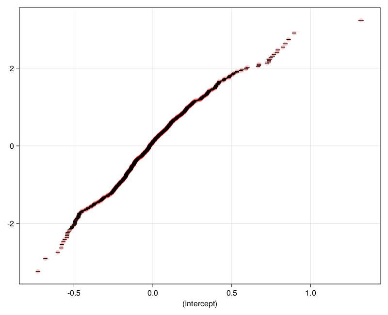
For the simple model elm01 the estimated standard deviation of the random effects for subject is greater than that of the random effects for item, a common occurrence. A caterpillar plot, Figure 12,

Code

qqcaterpillar!(
  Figure(resolution=(800, 650)),
  ranefinfo(elm01, :subj),
)

Figure 12: Conditional means and 95% prediction intervals for subject random effects in elm01.

shows definite distinctions between subjects because the widths of the prediction intervals are small compared to the range of the conditional modes. Also, there is at least one outlier with a conditional mode over 1.0.

Figure 13 is the corresponding caterpillar plot for model elm02 fit to the data with inaccurate responders eliminated.

Code

qqcaterpillar!(
  Figure(resolution=(800, 650)),
  ranefinfo(elm02, :subj),
)

Figure 13: Conditional means and 95% prediction intervals for subject random effects in elm02.

Random effects from the simple model related to covariates

The random effects “estimates” (technically they are “conditional means”) from the simple model elm01 provide a measure of how much the item or subject differs from the population. (We use elm01 because the main difference between elm01 and elm02 are that some subjects were dropped before fitting elm02.)

For the item its length and word/non-word status have already been incorporated in the model. At this point the subjects are just being treated as a homogeneous population.

The random effects conditional means have been extracted and incorporated in the byitem and bysubj tables. Now add selected demographic and item-specific measures.

itemextended = leftjoin(
  byitem,
  select(elpldtitem, 1:5);
  on = :item,
)
subjextended = leftjoin(
  bysubj,
  select(elpldtsubj, 1:3, :vocabAge);
  on=:subj,
)

814 rows × 11 columns (omitted printing of 2 columns)

	subj	ns	smiss	sacc	smedianrt	spropacc	elm01	elm02	univ
	Int16	Int64	Int64	Int64	Float64	Float64	Float64	Float64?	String?
1	1	3374	0	3158	554.0	0.935981	0.411459	0.426624	Morehead
2	2	3372	1	3031	960.0	0.898873	-0.30907	-0.293732	Morehead
3	3	3372	3	3006	813.0	0.891459	-0.153078	-0.139436	Morehead
4	4	3374	1	3062	619.0	0.907528	0.213047	0.22754	Morehead
5	5	3374	0	2574	677.0	0.762893	0.0850349	missing	Morehead
6	6	3374	0	2927	855.0	0.867516	-0.207356	-0.192651	Morehead
7	7	3374	4	2877	918.5	0.852697	-0.182201	-0.166357	Morehead
8	8	3372	1	2731	1310.0	0.809905	-0.541434	-0.526828	Morehead
9	9	3374	13	2669	657.0	0.791049	0.154926	missing	Morehead
10	10	3374	0	2722	757.0	0.806758	-0.0541104	-0.0403266	Morehead
11	11	3374	0	2894	632.0	0.857736	0.217734	0.231618	Morehead
12	12	3374	4	2979	692.0	0.882928	0.062351	0.0770981	Morehead
13	13	3374	2	2980	1114.0	0.883225	-0.409761	-0.3956	Morehead
14	14	3374	1	2697	603.0	0.799348	0.298338	missing	Morehead
15	15	3372	0	2957	729.0	0.876928	-0.00106274	0.0142299	Morehead
16	16	3374	0	2924	710.0	0.866627	0.0367131	0.0518282	Morehead
17	17	3374	1	2947	755.0	0.873444	-0.0599943	-0.0443423	Morehead
18	18	3374	0	2851	617.0	0.844991	0.223569	0.238685	Morehead
19	19	3374	0	2890	724.0	0.85655	-0.000190604	0.0147752	Morehead
20	20	3372	0	2905	858.0	0.861507	-0.169734	-0.155883	Morehead
21	21	3372	0	3051	1041.0	0.904804	-0.31294	-0.299952	Morehead
22	22	3372	2	2756	972.5	0.817319	-0.286105	-0.271354	Morehead
23	23	3374	3	2543	629.5	0.753705	0.25627	missing	Morehead
24	24	3374	0	2995	644.0	0.88767	0.165441	0.180714	Morehead
25	25	3372	0	2988	732.5	0.886121	-0.0395191	-0.0242025	Morehead
26	26	3374	0	3024	830.0	0.896266	-0.160068	-0.145719	Morehead
27	27	3374	1	2774	1099.5	0.82217	-0.32906	-0.314104	Morehead
28	28	3372	1	2898	823.5	0.859431	-0.179577	-0.164645	Morehead
29	29	3372	0	3022	1052.5	0.896204	-0.408285	-0.393552	Morehead
30	30	3374	0	2946	680.0	0.873148	0.0856058	0.0998801	Morehead
⋮	⋮	⋮	⋮	⋮	⋮	⋮	⋮	⋮	⋮

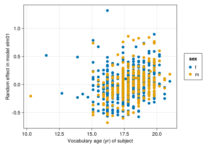
As shown in Figure 14, there does not seem to be a strong relationship between vocabulary age and speed of response by subject.

Code

draw(
  data(dropmissing(select(subjextended, :elm01, :vocabAge, :sex))) *
  mapping(
    :vocabAge => "Vocabulary age (yr) of subject",
    :elm01 => "Random effect in model elm01";
    color=:sex,
  ) * visual(Scatter)
)

Figure 14: Random effect for subject in model elm01 versus vocabulary age

Code

draw(
  data(dropmissing(select(subjextended, :elm01, :univ))) *
  mapping(
    :elm01 => "Random effect in model elm01";
    color=:univ => "University",
  ) * AlgebraOfGraphics.density()
)

Figure 15: Estimated density of random effects for subject in model elm01 by university

Code

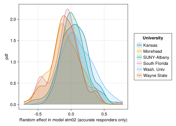
draw(
  data(dropmissing(select(subjextended, :elm02, :univ))) *
  mapping(
    :elm02 => "Random effect in model elm02 (accurate responders only)";
    color=:univ => "University",
  ) * AlgebraOfGraphics.density()
)

Figure 16: Estimated density of random effects for subject in model elm02, fit to accurate responders only, by university

Code

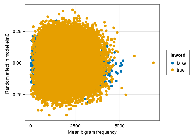
draw(
  data(dropmissing(select(itemextended, :elm01, :BG_Mean, :isword))) *
  mapping(
    :BG_Mean => "Mean bigram frequency",
    :elm01 => "Random effect in model elm01";
    color=:isword,
  ) * visual(Scatter)
)

Figure 17: Random effect in model elm01 versus mean bigram frequency, by word/nonword status

References

Balota, D. A., Yap, M. J., Hutchison, K. A., Cortese, M. J., Kessler, B., Loftis, B., Neely, J. H., Nelson, D. L., Simpson, G. B., & Treiman, R. (2007). The english lexicon project. Behavior Research Methods, 39(3), 445–459. https://doi.org/10.3758/bf03193014

Box, G. E. P., & Cox, D. R. (1964). An analysis of transformations. Journal of the Royal Statistical Society: Series B (Methodological), 26(2), 211–243. https://doi.org/10.1111/j.2517-6161.1964.tb00553.x